News

Integrated Engineering Software announces the release of Version 10 of its Electromagnetic Simulation Software programs. The new release provides you with notable performance improvements and with a range of new features for simulating Electromagnetic systems with hybrid solvers.

Enhancements in Version 10:

• There is a major interface upgrade with the introduction of a Model Manager that provides flexibility for completely new ways to control the program. This provides a simulation and application design environment that is customizable and can immediately accelerate your workflow upon integration, making it a worthwhile investment. There is a model tree in the workspace, allowing users to manipulate the visibility and view of the component model parts. Users can see the parts defined in the geometry model by expanding the tree nodes.
• Version 10 makes it more efficient to create models. Use of the newly developed "model search feature" allows built in access to an online library of models for your model formulation. This library will be expanded regularly. Users who wish to submit models for the library can contact support@integratedsoft.com.
• In addition to graphical modeling, INTEGRATED programs offer an Application Programming Interface (API) that is used to automate any repetitive modeling step. Version 10 has enhancements in API for designing high frequency and particle trajectory applications.
• During editing, particularly breaking and deleting, the Geometry ID numbers are renumbered which can be frustrating for advanced users. In Version 10, every geometry item has a permanent reference ID that will not change when another geometry is edited.
• Version 10 of INTEGRATED's 3D High Frequency Solver SINGULA features an integral equation solver based on the Multilevel Fast Multipole Method (MLFMM). This new solver can easily simulate large electrical structures, e.g. for Radar Cross Section (RCS) or antenna placement simulations.
  The advanced Boundary Element (BEM) settings in SINGULA now include “Levels” and “Box Size” settings for trading speed and accuracy for MLFMM. The higher the level of MLFMM, the faster the speed of the matrix vector product operations, and the lower the accuracy of the solution. The larger the box-size on the finest level, the slower the speed of the matrix vector product operations and the more accurate the solution. If the results of MLFMM are not obtained as expected, the user can adjust these settings. If the iterative method is not easy to converge, the user can increase the box-size at the finest level. If the results of MLFMM are not acceptable, the user can reduce the level of the MLFMM.
  Here are the default settings of the two parameters:
  

Online Information Session-Making Simulations More Efficient With Integrated 9.4

In this information session, Dr. Doug Craigen (Team-leader, Testing and Benchmarking, Integrated Engineering Software) presented the setup and solution of a variety of electric, magnetic and thermal sample models. This presentation highlighted the distinctive features of the INTEGRATED software, especially those introduced in version 9.4. These new features include a model search, graph window to model window interactivity, a new approach to grounding and voltage differences in electric solvers, and a breakdown of force and torque contributions in electromechanical problems.

Please watch the recording of online information session hosted by Integrated on August 15, 2017, here:

The most recent versions of INTEGRATED software programs feature a multi-criteria file search function. This enables users to search for keywords within Integrated.dbs files and examine the resulting matches in a preview pane before opening. Future versions will expand on the searchable criteria to include such properties as voltage sources, boundary conditions, program name (Electro, Coulomb etc.),  Dimensions (2D, 3D or RS) , Materials used, string in comment field, Size in Megabytes and outputs defined.

The following example will demonstrate the feature. Integrated.dbs files are distributed through several folders on drive C:\. The user can see all of those files simply by opening the search window, adding “C:\” as a search path and clicking the search button:

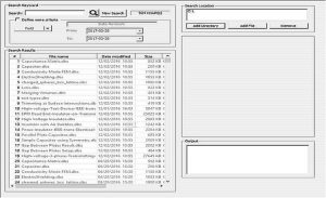
In this case, there are 924 results from the search. To refine the search, the user can enter a keyword, that is, some text used in a file comment, an object or material name, etc. A range of dates such as either the date the file was modified or the date of the program revision can also be added.

Then without opening every file, the user can select each resulting .dbs file and a preview image of the file, along with some information about the file, is displayed as shown below.

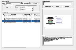
Note that the preview image is only contained in .dbs files saved in the V9.4 version and beyond. To convert any file to include this preview image, it is simply a matter of opening up the file in the latest version and saving it.

This version of SINGULA has some of the most promising features. With state of the art API scripting capabilities, SINGULA stands out among all simulation software. New advanced features will help minimize run time, hence increasing the feasible problem size by many folds. Some of the new features are listed below:

Exploiting symmetry to simplify modeling

• Planar symmetry can be utilized by users in the new version. It is extremely useful for modeling large systems to obtain a reduced model geometry. Now, symmetric/antisymmetric modelling can be applied on all the three principal planes.

Uniform Geometrical Theory of Diffraction (UGTD)

• The new version uses a hybrid method with the Method of Moments (MoM), Physical Optics (PO) and Uniform Geometrical Theory of Diffraction (UGTD). The Uniform Geometrical Theory of Diffraction (UGTD) is used for calculating diffracted fields from edges & wedges enhancing solution accuracy. This may be suitable for large parabolic reflective antennas.

More intuitive user interface

• User interface has been changed to make the program flow more user intuitive.

INTEGRATED is pleased to announce the latest version of CHRONOS, V9.4. With state of the art API scripting capabilities, the new list of advanced features will help solve all your FDTD problems. The release spotlights:

• Adaptive mesh refinements: The program generates the mesh once and can identify different materials in the computational domain. It will refine and regenerate the mesh automatically to fit the new structure.
• Post-processing of Z, Y, and S parameters for electric field and lumped voltage sources: The program can now calculate Z, Y, and S parameters between different antennas and microwave networks.
• Now the user can assign each of the following sources or loads along any arbitrary inclined directions:
  • E-field source
  • Voltage lumped source
  • Lumped load
  • Waveguide sources

The new version is extremely useful for modeling of lumped resistances, inductances, capacitances and infinitesimal delta voltage sources. Moreover, the program supports a comprehensive interface with the new version. Now, it is possible to create your own definitions for:

• The source table
• Conductors
• Lumped loads
• Delta voltage sources
• Electric field sources
• Current sources
• Planar ports/Ground
• Eaveguide sources
• Incident plane wave source

INTEGRATED Engineering Software will be attending CWIEME Chicago 2016 on October 4-5, 2016 which will take place at DE Stephens Convention Center, Chicago. We will be at Booth # H35.

This year, we are pleased to be able to offer complimentary passes to the show.

CWIEME Chicago is the meeting place for the transformer, electric motor and power generation industries in North America. The largest and most comprehensive event for the coil winding and electrical manufacturing sectors. CWIEME Chicago provides exhibitors with a unique opportunity to meet key buyers and decision makers across the Americas. It brings together visitors from over 1,100 motor and transformer manufacturing companies across the automotive, energy and consumer electronics, eager to find out more about the latest product developments and new suppliers in the market

INTEGRATED Engineering Software, a leading developer of hybrid simulation tools for design analysis, has introduced the INTEGRATED API (Application Programming Interface) across its simulation software suite with the release of the version 9.1 upgrade, providing a powerful scripting tool.

The INTEGRATED API, which enables smart automation scripting, provides design engineers with an intuitive method of controlling the interface. This supplements the existing interactive, parametric and batch modes. It provides users with direct access to the internal workings of each software program in the suite, enabling them to write new analysis applications specifically to meet their own needs and ability.

Through the INTEGRATED API, users can seamlessly connect their own applications to INTEGRATED software programs without either application requiring prior knowledge of the inner workings of the other. Design engineers, research scientists and programmers will find this a very powerful tool, combining good design with good performance, which enables them to complete tasks that would previously have been extremely difficult and tedious to do interactively.

“Our API enables design engineers and scientists to explore ideas and find new solutions with this custom analysis tool,” comments Bruce Klimpke, Technical Director. “Users will now have the power and flexibility to combine INTEGRATED’s CAE software programs with the applications they use for specific design analysis areas. This customization will allow each particular design to work at an even higher level of sophistication than previously.”

The INTEGRATED API also provides a key building block for users to construct custom analysis tools. The functionality is easy to explain and the names are self-explanatory and consistent, in order to drive development. A programmer can write a script, or a full program, describing how to build and analyze a specific problem with selected user controls, and can then invoke the INTEGRATED program direct through the API to provide the analytical tools.

Using the dedicated user guide included within the program, samples can be written as Excel VBA Macros or complete programs with Visual Studio solutions/projects.

Alongside the development and introduction of API features into the version 9.1 software release, INTEGRATED has included other new features within the upgrade, including:

• Much greater parallelization – as well as parallelizing the 2D BEM solver, there is more efficient use of parallel processing for the FEM solver and, in general, for post-processing operations
• Faster mesh generation – the time taken to generate an element mesh is now substantially reduced for many simulations
• Weighting factors – these can be used to inform the solver what areas are of special interest so it will produce especially good local results (fine element mesh)
• Auto solver- the auto solver setting will make the choice of FEM or BEM based on the general nature of the model. Either can still be manually forced
• CAD – new *.STEP/STP & *.SAT file import options; new geometry tools for healing common 3D CAD problems
• Geometry – the geometry now enables convenient names; new “block” option
• LORENTZ includes a new quasi-transient mode
• New mixed mode in OERSTED allows to establish effective permeability in nonlinear materials
• INDUCTO offers new heat/power source calculation
• CHRONOS now includes different methods of plane wave polarizations

Alongside this comprehensive software upgrade, INTEGRATED has developed its website to include a range of new demonstrative videos offering tutorials on the major new features in version 9.1, including API. These are available at Videos.

Chances are that if you’ve done simulation using Finite Element Method (FEM) or Boundary Element Method (BEM) software, at some point you’ve discovered or been told that your mesh was not adequate to obtain accurate results. At that point, you have two options available. You can globally increase the mesh density on your model, or you can use expertise and experience to search for areas on the model where an increased density would help the overall accuracy of the solution and then use tools available to mesh the model more finely in those areas.

Generally speaking, most organizations don’t have a meshing expert. In fact, in most organizations an engineer, physicist or designer includes computer simulation as only a small part of their duties. They have neither the time nor the desire to become experts in generating meshes for different types of simulation methods. For them, the ability of the simulation software to place an appropriate mesh on their model is critical. Additionally, if the application can show that it has converged to a stable result based on results from other meshes, they can have confidence in the simulation. This is where an adapting mesh becomes so important. In addition to saving the user time and effort in generating a mesh appropriate for obtaining accurate results, a proper adaptive mesh can also save solving time. By placing denser elements only where needed the most and making the mesh coarser where element density is not as critical, the size of the solution matrix and therefore the solving time is minimized.

Mesh Requirements for Boundary Elements and Finite Elements

The Boundary Element Method (BEM) is designed to reduce the dimensionality of meshing on physical models by one. That is, a two-dimensional (2D) model need only be meshed using one-dimensional (1D) elements on the outline of the model. For a three-dimensional (3D) model, 2D elements are only required on the surfaces of the model. In cases where volumetric source are applied or model materials have nonlinear properties, volume elements (2D elements for 2D models and 3D elements for 3D models) are required in those regions only. BEM solvers work especially well where there are large regions of open space because the field calculation is based on integrating over the boundary sources. Integration such as this provides a smoothing effect that differential methods sometimes force by applying smoothing functions.

Since the end solution of a BEM simulation is usually an equivalent source (currents or charges for electromagnetic solvers), the best accuracy is achieved when the mesh is fine enough to represent a relatively smooth variation in that equivalent source over the geometry. Where the equivalent source is relatively constant or linear, a coarser mesh is adequate. Finer meshes are required in areas where the source varies rapidly, generally at corners or where separate parts of the model come within close proximity to each other.

Using the Finite Element Method, the space is broken up in the same dimension as the model (2D elements for 2D models and 3D elements for 3D models). The finite element solution for electromagnetics usually consists of a scalar or vector potential at each node and fields are computed by calculating the derivatives of the potentials. Finer meshes mean that the variation in the potential can be more finely represented and therefore the field calculation by spatial differentiation of those potentials can be more accurately performed.

As with BEM meshes, FEM meshes can be coarser where there is a small variation in the solution, such as in large open regions. A finer concentration of elements is required in areas where the potentials, and hence the field, changes rapidly.

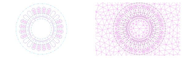Uniform Meshes of Boundary Elements (left) and Finite Elements (right) on a Permanent Magnet Motor Model in two dimensions.

Types of Elements for 2D and 3D

Common types of 2D elements are quadrilaterals and triangles. Analogously, common types of 3D elements are hexahedra, triangular prisms and tetrahedra. While structured finite elements, quadrilaterals and hexahedra, can be beneficial in solving FEM models from the point of solving efficiency, triangles and tetrahedra have the ability to conform to any proper closed model and the element size gradient throughout the model is easily changed. Triangles and tetrahedra are the preferred elements for self-adapting because they can be split simply by adding a point and swapping edges or faces. This kind of refinement can be done locally, whereas dividing a structured mesh may require propagating the division throughout an entire layer of the structure.

Adapting Elements for 2D and 3D Electromagnetics

The implementation of an adaptive meshing algorithm requires two phases.

The critical part of the process is determining where to refine the mesh. Any method used to measure the relative error in a solution must respect the physics of the simulation being performed. The solution gradient, itself, is a simple yet fast way to determine the local needs for mesh density in both the BEM and FEM. Also, if the mesh poorly represents the solution, errors in the fundamental field properties or satisfaction of boundary can be an indicator. For example, in the FEM solution to an electric field problem, the priority of elements to refine may be ordered by the magnitude of the difference in divergence of the D-field and the volumetric charge (normally zero) over each element. In the BEM solution to the same problem, the difference in the tangential E-field or the normal D-field at each element might be used to select which areas require a more dense mesh.

After determining where density in the mesh is required, the preferred method for generating the refined mesh for the next solution is to directly refine the existing mesh by inserting a number of points. Some algorithms will generate a density function to be used when generating the mesh from scratch. The density function in certain areas is increased at each step. By inserting points directly into the existing mesh, it is guaranteed that the elements with the greatest errors are refined. Using another refinement step after this to preserve a shape property will ensure that the transition between areas with a highly dense mesh and those with a more coarse mesh also contains well shaped elements.

A simple example is a parallel plate capacitor analyzed with interest in the electric fields. The field solution can be subsequently used to determine the total charge on the conducting surfaces which may be used to determine the stability of the solution. Using a BEM solver, the solution is a charge distribution on each plate – given an assigned constant voltage on each plate. Since the charge density is nearly constant on a large part of the capacitor plates, only few elements are required there. The charge density increases rapidly near the edges of the plates and therefore the most accurate solutions will have a very dense mesh at these edges. Similarly, for the FEM solution, the fields bend most at the corners of the plates and therefore the 3D mesh must be fine in those areas. In the center, between the plates and in the open space surrounding the capacitor, the field is relatively constant and therefore a coarse density is sufficient.

Adapted (left) and uniform (right) BEM meshes for parallel plate model with approximately the same number of elements.

Using the same general principles, the models with more complex electric field patterns such as a high voltage insulator can also be meshed adaptively

Section view of the adapted BEM mesh (right) of a high voltage insulator model (left).

By changing the type of physical guidelines for increasing the mesh density, the same general approach can be used for difference physical models. For example, using analogous magnetic field properties can be used to generate adaptive meshes for a variable reluctance sensor model or an eddy current model, such as a coil used for crack detection in metal surfaces.

Adapted FEM meshes on a variable reluctance sensor (left) and an eddy current nondestructive test coil sensor (right).

As an example of the efficiency and convergence of the adaptive process, a series of cogging torque calculations on the 2D permanent magnet motor model is performed using a FEM solver. Cogging torque can be a very difficult computation because it consists of an accumulation of very small forces acting in opposite directions. The calculated cogging torque for various numbers of elements using adaptive and uniform mesh distributions are shown in the graph below. With the adapted mesh, a stable convergence of less than 1% change is achieved after about 30 000 elements, while the uniform mesh solutions show greater fluctuations than this even after 100 000 elements. The case of over 400 000 uniform elements is included to confirm this.

Comparison of cogging torque calculations using adapted and uniform FEM meshes with similar number of elements

Using adaptive meshing gives simulation software users confidence in results and maintains efficiency in generating solutions and post-processing results. In electromagnetic simulation tools, refinement based on the solution and on fundamental field quantities are reliable ways to determine the areas of physical models where mesh refinement should be performed. This type of adaptive meshing places the expertise for mesh generation in the hands of the software and eliminates the need for mesh “tinkering” on the part of the software user.

Adaptive meshing is included in the suite of electromagnetic simulation tools from INTEGRATED Engineering Software for both 2D and 3D model simulations. All packages also include BEM and FEM solvers so users may choose the best method for their application. The presence of both kinds of solvers also provides and extra level of confidence, as users can compare results from each solution method to the other.

Speeds time to market for 3D RF and microwave applications

3D time-harmonic eddy current field solver was ahead of its time

Modeling and simulation of many RF applications and antennas present a challenge in terms of speed, required memory, and accuracy. For these applications if we move beyond using frequency domain techniques (e.g., boundary element method (BEM)) to time-domain solvers such as finite – difference time-domain (FDTD), huge savings in the running times are possible. The simple example of the conventional rectangular patch antenna, shown in Figure 1, shows the advantages of using our time domain solver. The problem was simulated in eight minutes using a single processor Intel(R) Xeon(R) 2.66 GHz to cover the frequency band 0.5 – 12 GHz, while the same problem should be simulated at 240 frequencies if a frequency domain solver is used. The running time for the simulation at each frequency using INTEGRATED’s frequency domain solver SINGULA (which is based on the Boundary Element Method (BEM)) was two minutes (total running time for the 240 frequencies was 8 hours).

To meet this challenge the company has introduced CHRONOS to its range of modeling and simulation software. The program is based on the Finite Difference Time Domain (FDTD) method, combined with an efficient mesh generator code and special treatments for arbitrary shaped and curved structures. This is ideal for a wide variety of RF and antenna applications and, being based on a direct solution of Maxwell’s equations in the time domain, has the following advantages:

• It provides a high accuracy for a wide variety of RF and antenna problems.
• No storage in time and no matrix inversion are needed.
• It gives the solution for broadband or ultrawideband problems from a single execution of the problem using a short pulse.
• It provides both of the near-field and far-field results from a single run.

Figure 1

Simulation of electrically large structures which have fine features, and general curved structures using the orthogonal FDTD mesh, is always challenging because of the heavy burden they impose on the CPU if the generated mesh is not optimized. For this reason CHRONOS has a smart mesh generator code with the ability to recognize all the details of any structure and decide how to distribute the mesh based on the accuracy requirements of the FDTD algorithm. This gives the user two options, to either generate the mesh distribution manually or automatically using the non-uniform smart mesh generator. The smart mesh generator is used to improve the accuracy of the solution and to reduce the number of cells used in the computational domain, leading to a significant improvement in the used memory and speed. The mesh is generated by placing finer grids in the areas which have fine features and then increasing the cell sizes gradually (to avoid spurious reflections) as the mesh moves away from these areas until the cell size reaches the maximum (usually λ/20) or it reaches near another region that needs fine a grid.

The problem shown in Figure 2 of a metamaterial antenna based on composite right/left hand (CRLH) [1] is a good example to show the advantage of using the adaptive grid generation. This metamaterial structure includes slots with widths of 0.2 mm and vias of radius 0.15 mm. The frequency of the first negative order resonance (n=-1) occurs at f=2.8 GHz as shown in Figure 2(b). The slot width is 0.001λ (at n=-1) and if a uniform grid is used with cell sizes in the x and y directions ∆x=∆y=0.1 mm , the number of unknown field components in the computational domain is 15.6 million while using adaptive grid reduces the number of unknown field components to 5.7 million.

Figure 2a
Figure 2b

Figure 3 shows the problem of the electromagnetic penetration in a building with dimensions 7m x 10m x 10 m. The building is located at a distance of 3m from an antenna resonating at 1 GHz. The total dimensions of the problem are 7m x 13m x 10m and after adding additional spaces to the absorbing boundary conditions, the problem requires 1.1 billion of unknown field components to be simulated. The running time for this problem was 51 hours and 44 minutes using Intel(R) Xeon(R) E5430@2.66 GHz (2 processors) with 48 GB RAM and 64 bit operating system. Figure 4 shows the distribution of the electric field component Ez at f=1 GHz in the y-direction along the central line of the first floor and the central line of the second floor.

Figure 3
Figure 4

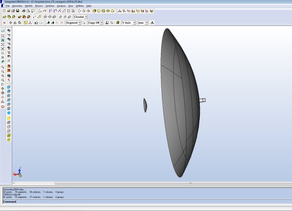
Although the above examples show several advantages in using the time domain solver, using a frequency domain solver such as SINGULA has big advantages when solving large electromagnetic problems, especially when the simulation is required at only a few frequencies. Solving large problems that have largest dimension about 100λ is difficult using Boundary Element Method (BEM) / Method of Moments (MoM). For solving such large problems, the Fast Fourier Transfer (FFT) technique was incorporated into the BEM. Figure 5 shows a large Cassegrain parabolic reflector antenna fed by a conical horn radiating a circularly polarized pattern [2]. The focal length and the aperture diameter of the main reflector (paraboloid) are F=1.221m and D=3.8m. The parameters, distance between the foci and the aperture of the hyperbolic subreflector are 1.221 m and 0.3042 m, respectively. Simulations were carried out at a frequency of 10GHz (126.6λ).

Figure 5

Though MoM has many advantages over FEM for the open region electromagnetic field problems, FEM can offer faster solutions for the closed region problems with almost the same solution accuracy as that of MoM. This fact is even more relevant in the determination of the global parameters such as Z, Y, and S matrices of RF circuits. Another application, where FEM can be a better choice, is the determination of the eigenvalues of the microwave resonators of arbitrary shapes. In view of these advantages, FEM solver is also incorporated in our high frequency electromagnetic field solver SINGULA.

As a conclusion, the time domain solver CHRONOS is much faster than the frequency domain solvers especially when the solution is required over a wideband of frequencies, while the frequency domain solver SINGULA gives advantages for solving very large problems when the simulation is required at only a few frequencies or at a single frequency. With the development of CHRONOS, the most powerful innovative techniques of Finite Difference Time Domain, Method of Moments (MoM), and the Finite Element Method (FEM) will be available to the designers in the Integrated’s Software environment [3].

References:

[1] Hany E. Abd-El-Raouf, et al., “Design of Double Layered Metamaterial Antenna,” Eucap 2009 3rd European Conference on Antennas and Propagation – 23-27 March 2009 in Berlin, Germany.

[2] “Simulation of Large Cassegrain Reflector Fed by Point Source in SINGULA”, www.integratedsoft.com, April 2010.

[3] Tom Judge, “Adaptive BEM and FEM meshing increase confidence in electromagnetic simulation results”, Bodo’s Power System, pp.38-40, December 2009.

One of our major developments over the last two years was the multi-threading or parallelization of the 3D programs. Users of the software often got results in minutes as opposed to hours using dual quad core machines. This was especially true for the boundary element method where the process of generating the system matrix and right hand side of the governing integral equations lends itself ideally to parallel processing. In addition, the dense matrix resulting from the boundary element method could be multi-threaded as well. Of course, what sounds simple to do was in fact quite challenging as the complete data structure of parallel algorithms is far more demanding than simple serial computing.

This development will now be the basis for implementing the same data structures and program implementation for the 2D programs. Although the benefit of parallel computation will perhaps not be as significant as experienced by 3D users, the speed improvement will certainly be a major plus. The speed increase will initially be found with the boundary element solver. However, some of these methods will eventually be used to the finite element software for mesh and matrix generation. We look forward to this development in V9.1.

Figure 1 Cassegrain reflector with conical horn feed.

In many reflector antenna applications, it is convenient to simulate the reflector system fed by a point source whose far field radiation pattern is same as that of the actual feed used in the application. Point sources with the user specified far zone E-field radiation patterns can be input as excitation source in SINGULA. The E-field radiation pattern of the point source can be specified in any one of the three ways provided in the program.

The first way is by selecting from the list of the standard far zone patterns available in the program. This list contains "Isotropic Source", "Z-Directed Electric Hertzian Dipole", "Z-Directed Elementary Magnetic Dipole", "Gaussian Beam", etc..

The second way is by specifying the far zone radiation pattern in a functional form given by

where the function F(θφ) is the pattern of the Eθ component and the function G(θ, φ) is the pattern of the Eφ component. As an example, a scalar feed can be defined in a simulation by specifying F(θφ) and G(θφ) as

F(θφ) = exp(-θ^2)*cos(p); G(θφ) = exp(-θ^2)*sin(p)

The list of valid operators and different functions allowed to use in the functional form of the point source along with their syntax are given in the manual.

The third way of defining the far zone radiation pattern of the point source is by specifying it in a tabular form in the format given below.

Φ(deg.), θ(deg.), | Eθ | (V/m), Angle Eθ(deg.), | Eφ | (V/m), Angle Eφ (deg.)

The data file containing the E-filed data recorded in the above specified format can be read in SINGULA for defining the far zone radiation pattern of the point source in a simulation. The E-field of the point source in any arbitrary θ , φ direction is calculated by a linear interpolation of the E-field values specified in the table.

The third way of defining point source in Singula is useful only if the far zone E-field values in the required φ, θ range are already recorded in a data file in the above specified format. Measured 3D-radiation pattern of the feed antenna recorded in a data file in the above specified format can be read directly in SINGULA for defining the point source. Also, the 3D far zone E-field pattern of a feed antenna simulated in SINGULA can be output to a file which can be read as a far zone E-field pattern of an equivalent point source for the subsequent simulations. This feature is very useful for analyzing the large reflector antennas and/or the large conducting scatterers. However, two simulations are required in SINGULA to handle this type of problems. First the feed antenna alone, centered at the origin of the global XYZ-coordinate system, is modeled and solved. The 3D far zone E-field radiation pattern of the feed antenna thus obtained is output to a file which may arbitrarily be named as 'Feed Pattern'. Then the reflector antenna system alone is modeled as a separate simulation in which the reflector system is illuminated by a point source whose 3D far zone E-field radiation pattern is read from the file 'Feed Pattern'.

Large reflector antennas are difficult to simulate using Boundary Element Method (BEM) / Method of Moments (MoM). However, incorporation of the Fast Fourier Transfer (FFT) technique into the BEM makes the simulation of large reflector antennas practical. Here, a large Cassegrain parabolic reflector antenna fed by a conical horn radiating a circularly polarized radiation pattern is considered to illustrate the validity of the use of an equivalent point source as a feed. Simulated radiation patterns of a Cassegrain reflector antenna, fed by the conical horn radiating circularly polarized wave, are compared to that of the same Cassegrain reflector fed by the equivalent point source having the radiation pattern of the same conical horn feed under consideration.

The geometry of the Cassegrain system, employing a concave paraboloid as the main reflector and a convex hyperboloid as the subreflector is shown in Fig. 1. The focal length and the aperture diameter of the main reflector (paraboloid) are 1.221m and 3.8m, respectively. The parameters , distance between the foci and the aperture of the hyperbolic subreflector are 1.221 m and 0.3042 m, respectively. These specifications imply the semi-major axis a and the semi-minor axis b of the hyperbola, whose surface revolution yields the subreflector, are 0.5m and 0.3503m, respectively. The main and the subreflectors are positioned such that the real focus of the hyperbolic subreflector is aligned with the vertex of the main reflector and the virtual focus of the subreflector with the focus of the main reflector. The phase centre of the conical horn feed is aligned with the vertex of the main reflector for illuminating the subreflector. The dimensions of the conical feed horn are shown in Fig. 2.

Figure 2 The circular horn fed by two orthogonal TE11 waveguide modes.

In the first phase of the simulation, the conical horn is fed by two orthogonal TE11 circular waveguide modes at the beginning of the cylindrical section of the feed horn to generate a circularly polarized radiation from it. After solving the model in SINGULA the phase centre of the feed horn and the 3D E-field radiation pattern at a resolution of 0.2° in the θ-direction and 2° in the φ- direction are obtained. In the program, the angular range for the 3D E-field radiation pattern is set 0°-50° for θ and 0°-360° for φ . The data calculated by the program to draw the 3D pattern can be recorded in a file simply by clicking on the "Export" button designated for this purpose in the user interface of the program. Simulations were carried out at frequencies of 3GHz, 6GHz, and 10GHz. The 2D polar patterns of the directive gain of the conical feed horn in the principal planes at these three frequencies are shown in Figs. 3-5.

Figure 2 The directive gain pattern of horn at 3GHz and 6GHz

Figure 4 The directive gain pattern of the conical feed horn at 10GHz

In the second phase of the simulation, the Cassegrain reflector system fed by the conical feed is modeled and solved. In the third phase of the simulation, the Cassegrain reflector is illuminated by an equivalent point source whose radiation pattern is defined by the data files of the feed 3D E-field patterns obtained in the first phase of the simulation. The far zone radiation patterns thus obtained in the second and third phases of the simulation are compared in Figs. 5-10.

In Figs. 5-10, simulated results obtained by different methods for different models are compared. The short legends appear in these figures are explained below.

"LU, single precision" ----- Cassegrain reflector fed by the conical horn solved by single precision LU decomposition method.
"FFT" -------- Cassegrain reflector fed by the conical horn solved by iterative method with FFT technique.
"PS-FFT" ------ Cassegrain reflector fed by the equivalent point source by iterative method with FFT technique.

Figure 5 The directive gain pattern in φ=0° plane at 3GHz Figure 6 Left Hand Circular Polarization (LHCP)-component pattern of far-zone E-field in φ=0° plane at 3GHz. Figure 7 The directive gain pattern in φ=0° plane at 6GHz Figure 8 Left Hand Circular Polarization (LHCP)-component pattern of far-zone E-field in φ=0° plane at 6GHz.

From these illustrations, we can observe close agreement between the radiation patterns of the Cassegrain reflector with the conical horn as feed and with the equivalent point source as feed. Fig. 10 and 11 are the radiation patterns of the Cassegrain reflector illuminated by the equivalent point source obtained using iterative method with FFT technique.

Figure 9 The directive gain pattern at 10GHz. Figure 10 The LHCP-component pattern of far-zone E-field at 10GHz.

INTEGRATED’s applications are moving more toward providing analysis from multiple solutions, such as transient analysis and time domain analysis. For these types of applications, users will feel the need to define the kinds of calculation and output they want to see at each step before generating the solutions. This will make generating useable results work more smoothly and quickly once the analysis is finished. INTEGRATED is, therefore, introducing a new interface for pre-defining plots and calculations to be performed after each solution step and an interface to manage and plot these outputs using animations, step-through plots and graphs of calculated values.

The process of working with multiple step plots and calculations involves two steps.

The pre-solving step is the Define Output process, where plots and results are defined. This will instruct the application which calculations will be performed after each solution step. Users will pre-define the output through the Define Output interface:

The Plots tab on this dialog is for defining the plots (contours, arrows, etc.) to be generated at each solution step. Selecting “Add Plot” allows you to define a new plot. Plot Properties are set in a tabbed dialog, designed to let you find the kind of plot you want more easily and intuitively.

The Results tab allows you to define single value calculations such as forces on parts, power loss on structures, or the field values at some point in space.

Many different plots and results can be defined and then activated or deactivated to save time in the overall analysis. Each plot and result is named for easy reference.

After solving, all of the data for the requested plots and results are accumulated. You can then use the Output Manager to generate animations of multiple plots or step through the plots over the range of the transient analysis.

You can also use the Output Manager to generate graphs of single value calculations against the transient time step or display a table of the results for the analysis.

The Transient Analysis mode available in ELECTRO, OERSTED, and KELVIN has the capability to create virtually any desired time dependent source with a library of Standard signals, an algebraic Function editor, and the ability to read in Tables from text files.

Standard Signals

Often the desired source can be constructed by using one or more of the Standard predefined time signals.

Examples of the Standard time signals available are shown below. These signals are typical of the type found in mathematical handbooks.

Once you’ve selected a signal from the drop down list, you can set the relevant parameters for the signal in the numeric field boxes. Below we show an example of a Periodic Triangular Pulse Source that is defined by four parameters; a Start time, an Amplitude, a Pulse width and a Period (if desired a fifth parameter, Stop time, could also be specified).

Graphs of the time variation of the source can be plotted using the [Plot Source] button. The [Plot All] button produces graphs of all component signals in addition to the resultant source.

For the parameter settings given above, the source will be the time function shown in the plot below.

Function Signals

You can enter signals as closed form functions of time by selecting the Function radio button and entering the signal as an algebraic expression. An example of this is shown below.

A plot of the resulting signal is shown below.

Note that the arguments of trigonometric functions are assumed to be in degrees. Also note that there should be no extra spaces in formulas as these will cause parsing errors.

Table Defined Signals

As a final option, you can define signals by creating text files containing two-column data tables.

In the example shown below, the first column represents discrete time instants, and the second column represents the corresponding signal values. Note that the data points describe a signal with zero initial value followed by a positive pulse of 0.4 starting at t=0.25 and lasting till t=0.5. After another zero interval, a negative pulse of -0.2 starts at t=0.8 and lasts until t=0.9. The signal then returns again to zero.

Below we show the Component Signal Properties section as it appears when the Table radio button is selected. Click the file open button to locate to the desired data file. Note also that the Linear radio button has been selected in the Interpolation section.

The resulting time signal is shown below. Note that Linear interpolation should be used for signals with sharp transitions, but Nurbs should be used for continuous signals.

The question is often asked “Which is the better technology: Boundary Element Method or Finite Element Method?” The answer to this question depends on the problem you are solving. For some problems, BEM has huge advantages over FEM and the opposite can be said as well. The best way to look at this is to review both methods for electric, magnetic, and thermal calculations.

There are a wide range of electric problems that arise. Some involve only the permittivity, others the conductivity, and for many problems both properties need to be considered in the calculation. Often for the case where the conductivity can be ignored and only the permittivity considered, we are dealing with problems where there is a large exterior region. If we consider a high voltage insulator attached to a power line, the huge open space (infinite actually) around this structure has to be included in the model. The Boundary Element Method does this naturally with no additional unknowns required. Theoretically, we can calculate the fields at infinity (zero in 3D of course) using the BEM approach. If we attempt to solve this problem using FEM we have to artificially truncate the problem by typically placing the structure in some finite box. The number of finite elements required in the space surrounding the structure can be huge. On the other hand, if we are solving a nonlinear conductive problem, where the space surrounding the conductive region is ignored, the FEM has huge advantages speed wise. Clearly for electrical problems, having both methods available can be very advantageous.

Similar situations arise for magnetic problems. Often, for problems involving magnetic sensors, there is a lot of free space around the sensor. For these applications the BEM is preferred as the free space is taken care of automatically. Also, for problems where extreme accuracy is required the BEM can often deliver where it may be almost impossible to achieve acceptable results using FEM. For highly nonlinear motor applications, where the external region is of no consequence, the FEM approach is definitely the method of choice.

For thermal applications boundary conditions must encompass the entire region. Therefore, unlike electromagnetic problems, finite elements are almost always the favored form of solution.

Boundary element analysis of an artificial heart pump – Courtesy of University of Nottingham

Now we will get down to the real benefit of having both FEM and BEM. For any real world application there is a unique solution. So independent of the method used to achieve the solution, the results should closely approximate the real world results. The question the user always has is “How good are my results?” The results of the two methods of simulation (BEM and FEM) can be compared. If they match reasonably well the user can be quite assured that the simulation data is correct. This is a very powerful method of verification of results that is of course, only available if both methods of simulation are present.

In conclusion, having FEM and BEM available in the same software has two main advantages; the right technology can be applied for the given problem and the results of both methods can be compared to assure the user that the answers are in fact correct.